KV Caching Illustrated

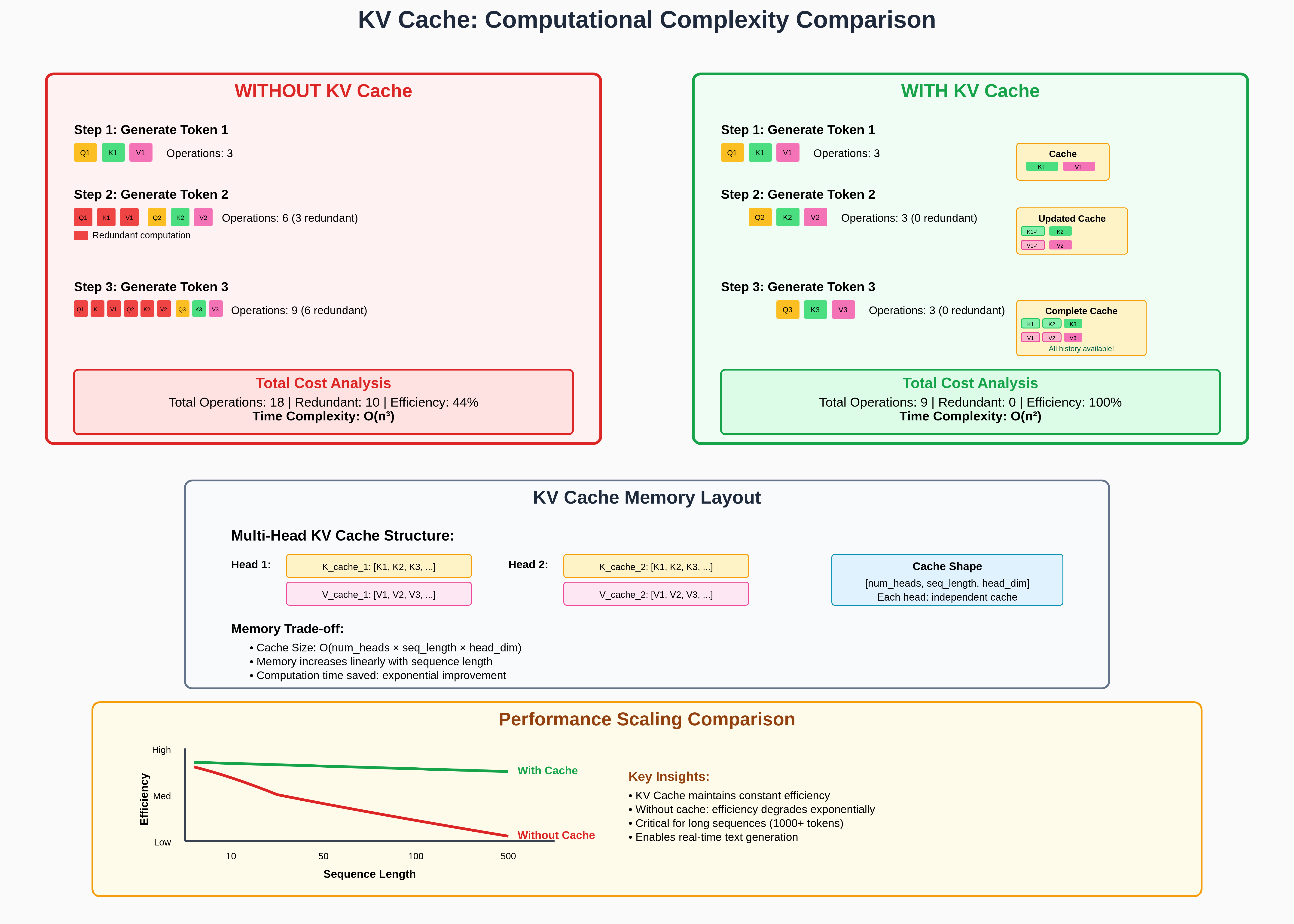
KV Caching is an optimization technique used during inference in transformer models to avoid redundant computations of Key (K) and Value (V) matrices for tokens that have already been processed. This dramatically speeds up autoregressive text generation.

Example Setup

Let’s use a simple example:

• Input sequence: “The cat sits”
• Vocabulary: {The: 1, cat: 2, sits: 3, on: 4, mat: 5}
• Model: 2 attention heads, embedding dimension = 4
• Sequence length: 3 tokens

---

Training Phase

Input Embeddings

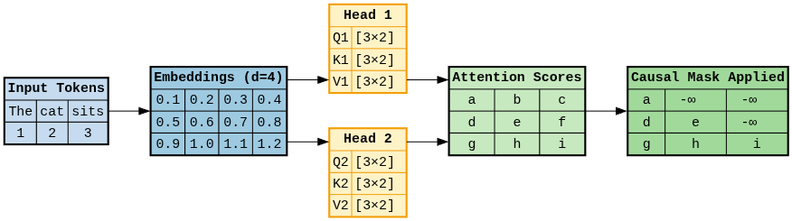
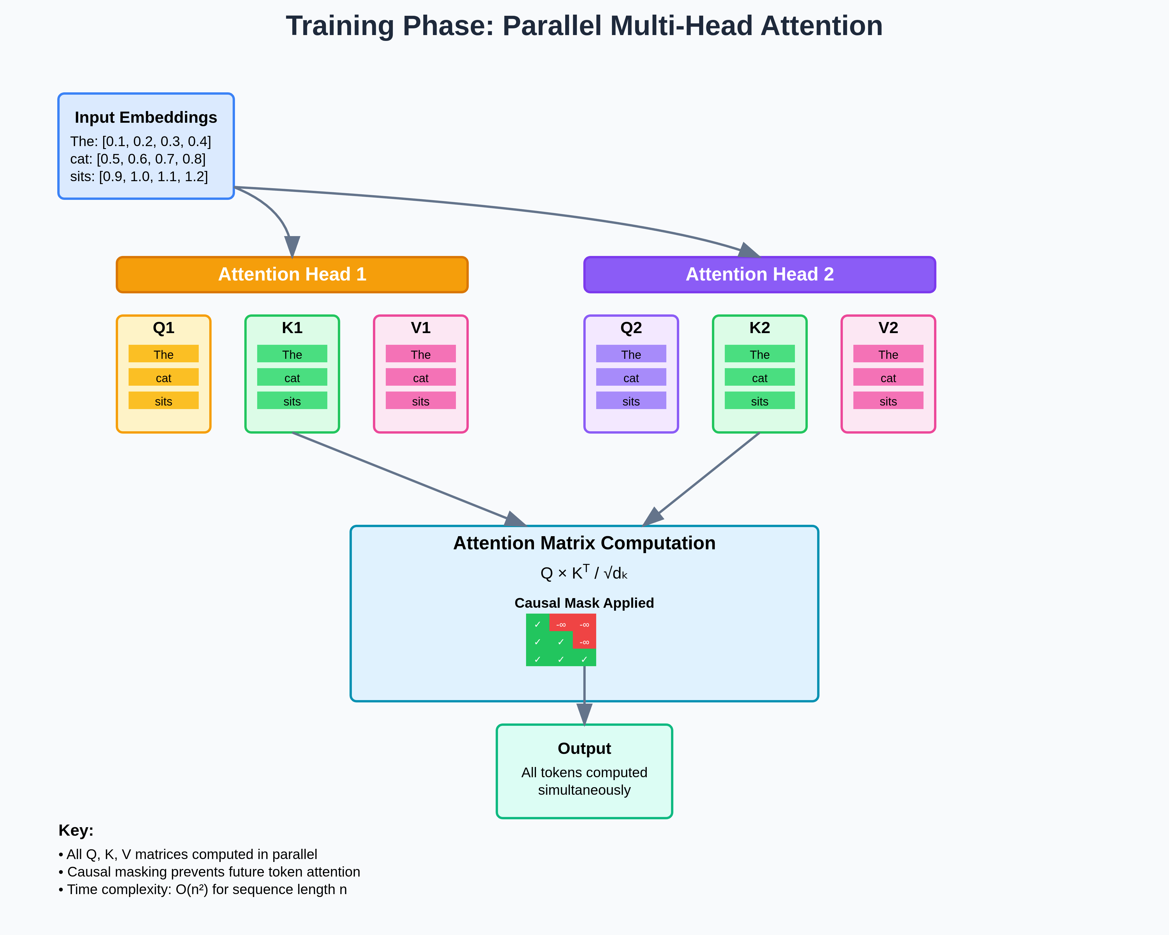
Tokens:     ["The", "cat", "sits"]
Token IDs:  [1, 2, 3]
Embeddings: 
  The:  [0.1, 0.2, 0.3, 0.4]
  cat:  [0.5, 0.6, 0.7, 0.8] 
  sits: [0.9, 1.0, 1.1, 1.2]

Multi-Head Attention Computation

Attention Matrix Computation:

\(\begin{align} Q &= XW^Q \\ K &= XW^K \\ V &= XW^V \\ \text{Attention}(Q,K,V) &= \text{softmax}\left(\frac{QK^T}{\sqrt{d_k}}\right)V \end{align}\)

For each attention head, we compute Q, K, and V for all tokens in the sequence simultaneously. This is because during training, the model processes the entire input sequence in parallel, rather than one token at a time (as in inference with KV cache).

Let’s assume we have 3 tokens in the input sequence, each represented by an embedding vector, and each head projects them into a lower-dimensional space (d_k = 2 in this example).

NOTE: For each head, we compute Q, K, V for ALL tokens simultaneously

Head 1:

Q1 = Embeddings × W_Q1    # Shape: [3, 2] (3 tokens, 2 dims per head)
K1 = Embeddings × W_K1    # Shape: [3, 2]
V1 = Embeddings × W_V1    # Shape: [3, 2]

• Embeddings: A $[3, d_{model}]$ matrix (3 tokens, each of dimension $d_{model}$).
• $W_{Q1}$, $W_{K1}$, $W_{V1}$: Learned projection matrices, each of shape $[d_{model}, d_k]$.
• Multiplying embeddings with these weights projects the input sequence into head-specific query, key, and value representations.
• Output shape [3, 2] means: 3 tokens × 2-dimensional vectors per token (per head).

Head 2:

Q2 = Embeddings × W_Q2    # Shape: [3, 2] 
K2 = Embeddings × W_K2    # Shape: [3, 2]
V2 = Embeddings × W_V2    # Shape: [3, 2]

Same process, but with different parameter sets ($W_{Q2}$, $W_{K2}$, $W_{V2}$) unique to Head 2.

Each head learns its own way of “looking at” the input sequence.

Attention Scores & Masking

Once we have queries and keys, we compute similarity scores between every query token and every key token.

• Q has shape [3, 2] and $K^T$ has shape [2, 3], giving a [3, 3] matrix.
• Each row corresponds to one query token comparing itself against all 3 keys.
• Division by sqrt(d_k) (here, √2) scales the dot products to avoid overly large values that would destabilize softmax.

Causal Masking Applied:

Before masking:     After masking:
[[a, b, c]    →     [[a, -∞, -∞]
 [d, e, f]           [d,  e, -∞]
 [g, h, i]]          [g,  h,  i]]

• Before masking: every token can attend to every other token.
• After masking: we enforce causality by preventing a token from attending to future tokens.
  • Example: token 1 can only attend to itself (a), not token 2 or 3 (set to -∞ before softmax).
  • This ensures autoregressive training — each token learns to predict the next one using only past and current context.

---

Inference Processing

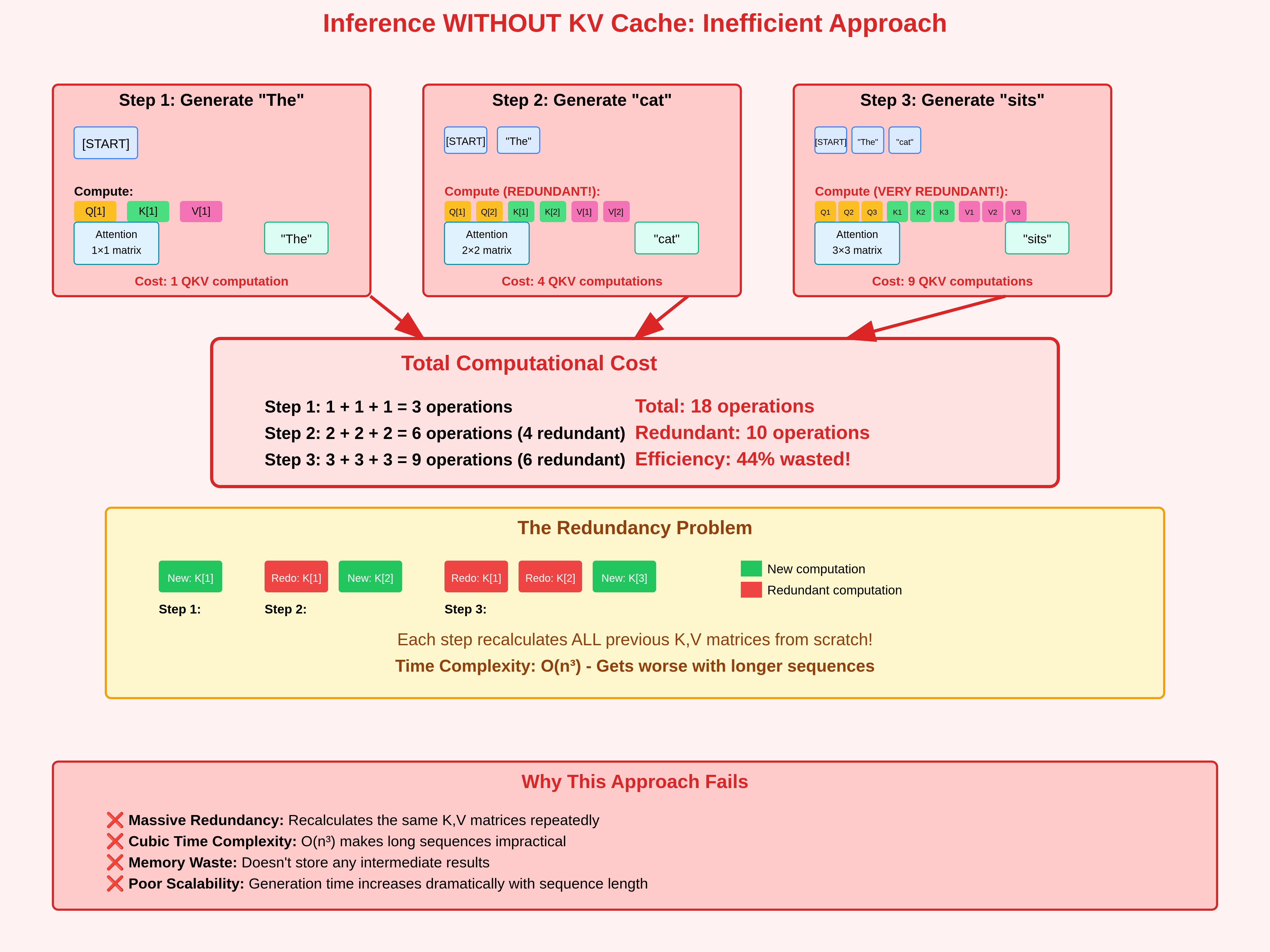
Inference Without KV Cache (Redundant Work)

When generating tokens autoregressively, the model predicts one token at a time. At each new step, it needs the current query $Q$ and must attend to all past tokens via $K$ and $V$.

Token 1 (“The”):

• Compute $Q_1, K_1, V_1$ for position 1.
• Attention is trivial (self-attention with just one token).

Token 2 (“cat”):

• We need $Q_2$ for the new token.
• But without caching, we also recompute $K$ and $V$ for both token 1 and token 2, even though $K_1$ and $V_1$ were already computed in the previous step.
• This is the first layer of redundancy.

Token 3 (“sits”):

• Again, we need $Q_3$ for the new token.
• But without caching, we recompute $K$ and $V$ for all three tokens (1, 2, 3).
• Now we’ve wasted effort: $K_1, V_1, K_2, V_2$ were already computed in earlier steps, but are recalculated from scratch.

---

Why Is This Redundant?

• Queries ($Q$) must always be recomputed: each new token has a new query that defines what it wants to look at.
• Keys and values ($K, V$) do not change for past tokens: once a token is embedded and projected, its representation stays fixed.
• Recomputing them at every step is unnecessary — we already know their values from earlier steps.

---

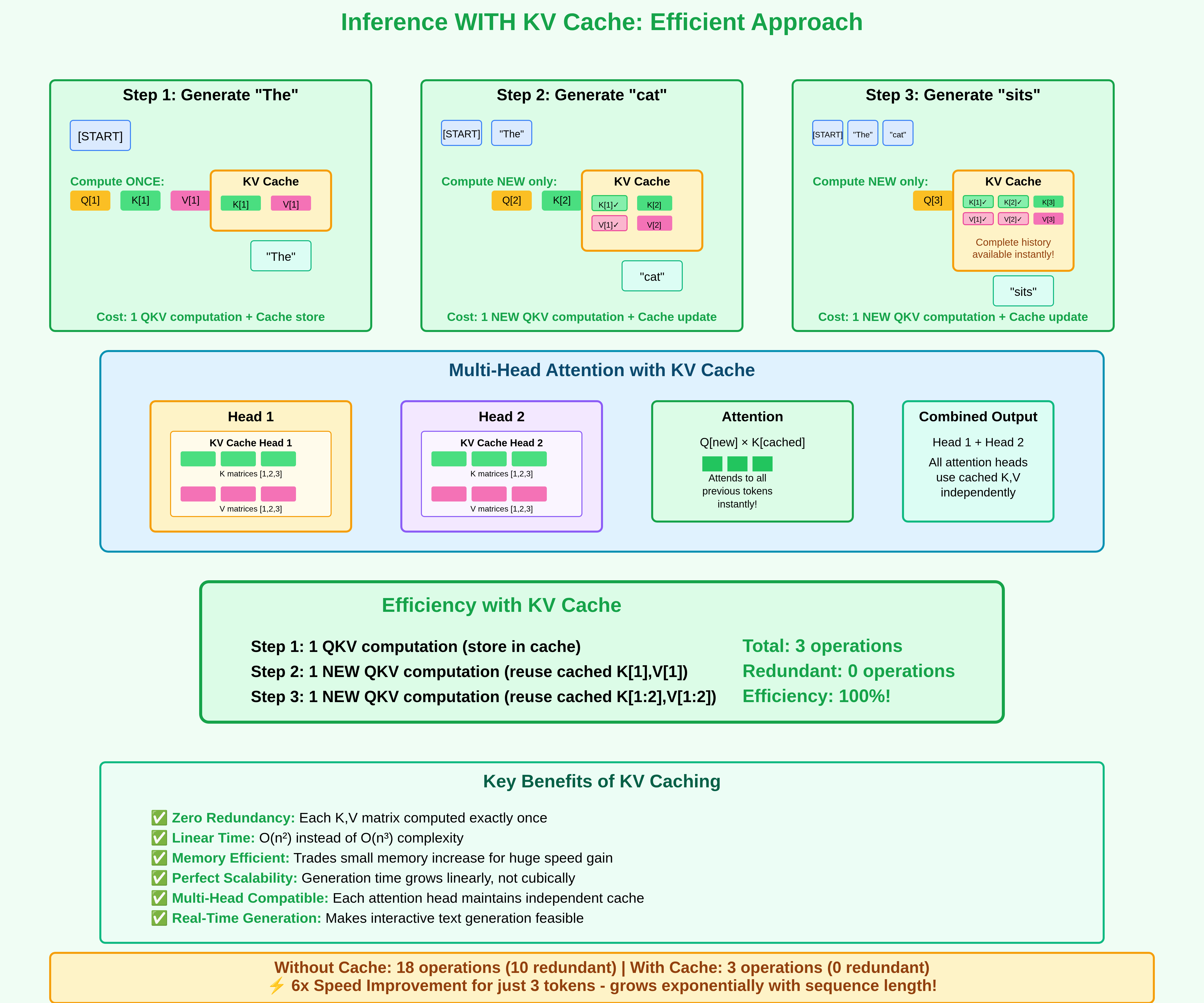
Solution: KV Cache

Instead of recomputing, we store $K$ and $V$ for all past tokens in a cache.

At step $t$, we only compute:

• $Q_t$ for the new token
• $K_t, V_t$ for the new token (to append to the cache)

Past $K$ and $V$ are reused directly from the cache.

This reduces the computation at each step from $O(t \cdot d)$ (recomputing for all tokens) to $O(d)$ (just for the new token).

Summary

In this post, we showed exactly how redundant computations are eliminated while calculating QKV matrices during attention calculation and why KV caching is essential for modern language models. Without it, generating long sequences would be computationally prohibitive!